A Practical Guide to Traceroute (tracecrt)
Richard Steenbergen
- 7 minutes read - 1290 wordsTraceroute is the first tool most of us reach for when something on the network misbehaves, yet it is also one of the most frequently misread. A single hop that looks “slow” might be a rate-limited ICMP response, not a real latency problem. A path that appears to jump between continents might just be an asymmetric route. Understanding what traceroute is actually doing under the hood turns it from a guess into a diagnostic.
📎 Download ras-traceroute-n45.pdf
Introduction
Troubleshooting problems on the Internet and enterprise networks often starts with a traceroute. But what is actually wrong with the way most people read traceroute output? The short answer: they treat every hop as a real network device and every millisecond as a real delay. In practice, many of the hops you see are artifacts of how routers handle TTL expiration, rate-limiting, and MPLS encapsulation.
How Traceroute Works
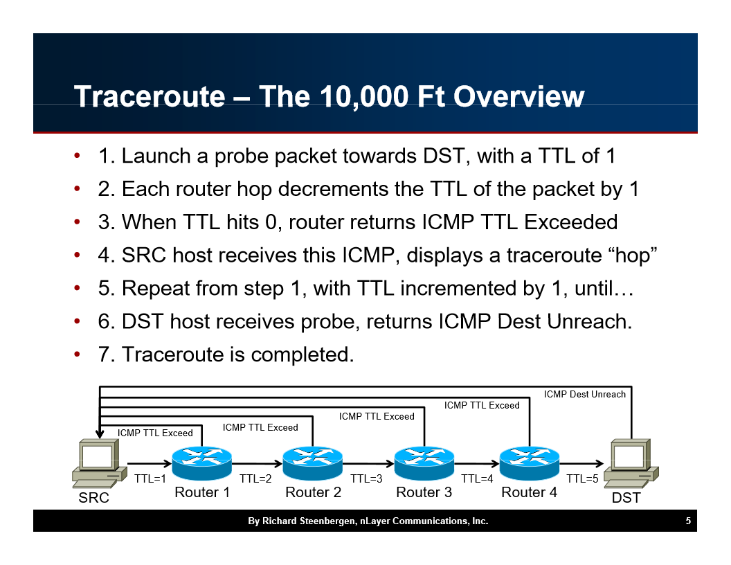
At its core, traceroute sends a series of probes with incrementing TTL values. Each router that decrements the TTL to zero returns an ICMP Time Exceeded message, which reveals its identity. The final destination returns an ICMP Port Unreachable (for UDP probes) or an ICMP Echo Reply (for ICMP probes), signaling the end of the path.
Multiple Probes
Most traceroute implementations send three probes per hop. This gives you a small sample of latency and helps identify packet loss. However, three samples is a very small statistical set, so treat the numbers as indicative rather than definitive.
Traceroute Latency Calculation
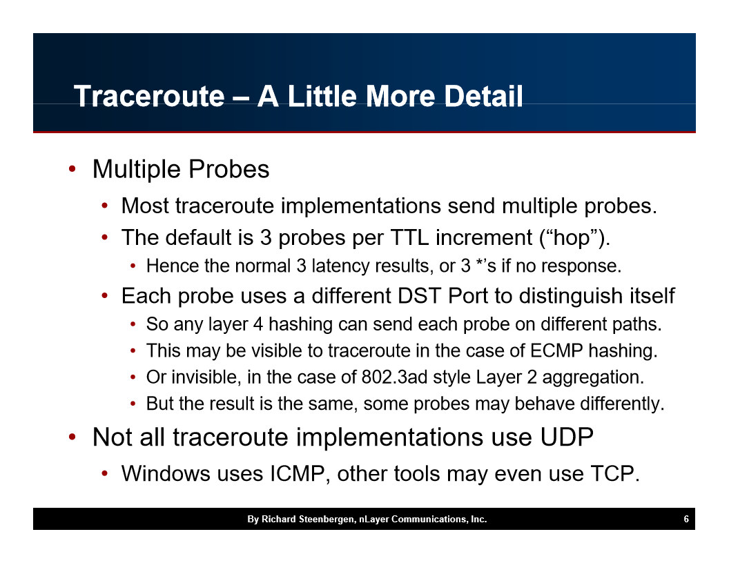
The latency you see at each hop is the round-trip time for that specific probe. It includes serialization delay, propagation delay, and queuing delay at every router along the path. A high number at one hop does not necessarily mean that hop is the bottleneck; it may simply be the first router that is slow to respond to the TTL-exceeded message.
What Hops Are You Seeing?
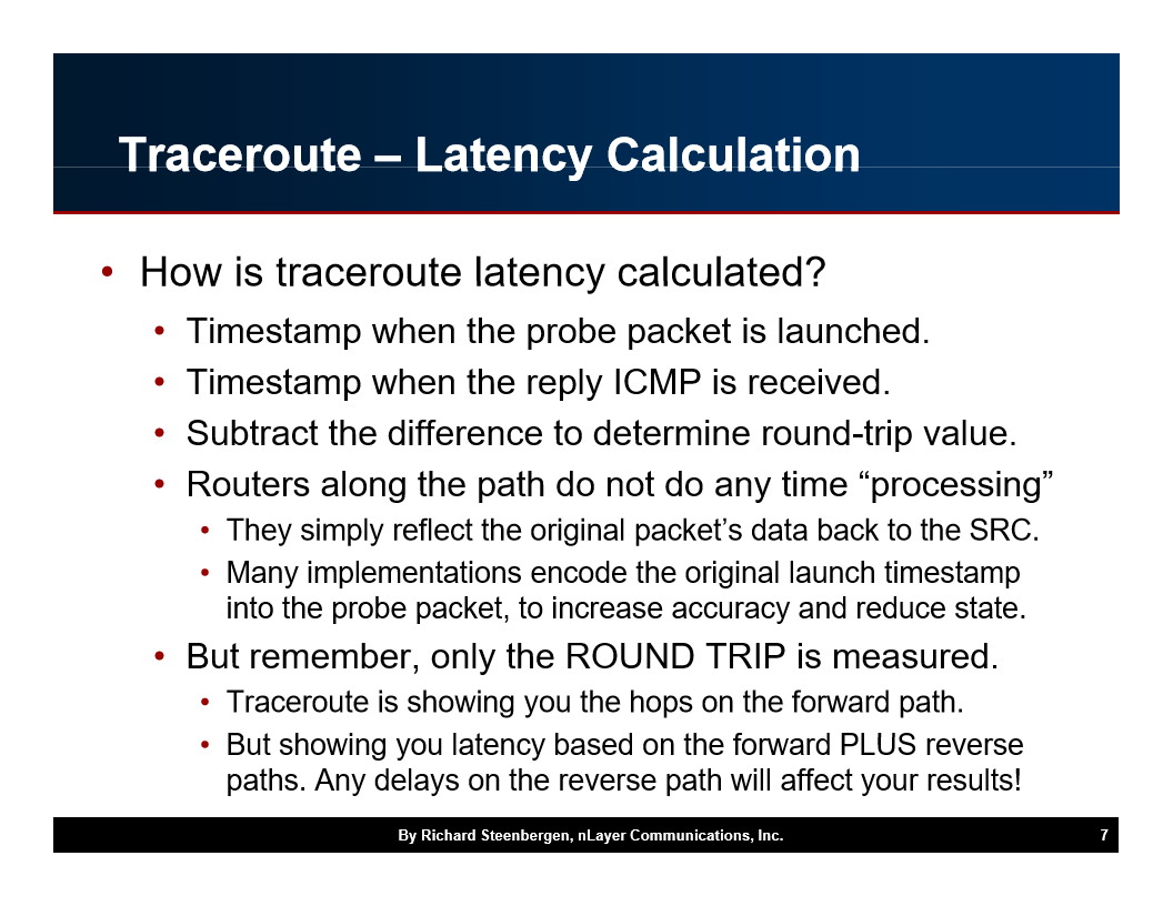
Each hop in the output corresponds to a router (or a virtual interface on a router) that generated the ICMP Time Exceeded reply. In MPLS networks, you may see the same physical router appear multiple times because each MPLS label push or pop can create a separate logical hop.
Interpreting DNS in a Traceroute
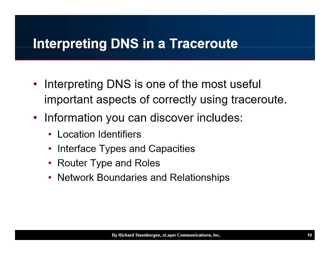
Reading the reverse-DNS names (PTR records) attached to each IP address is one of the fastest ways to understand what you are looking at.
Knowing the Geographical Location
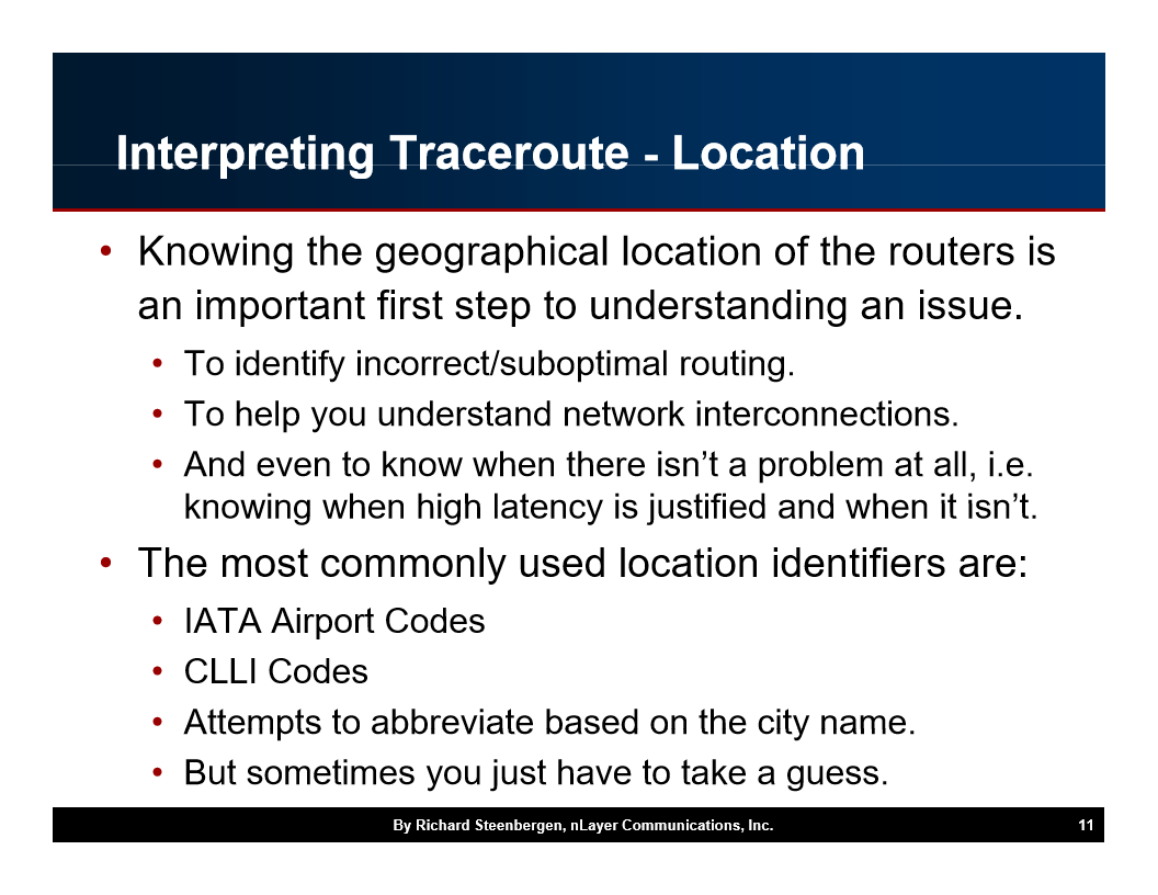
Many operators encode the datacenter location in the hostname. Common patterns include city names, IATA airport codes, and internal location identifiers.
IATA Airport Codes
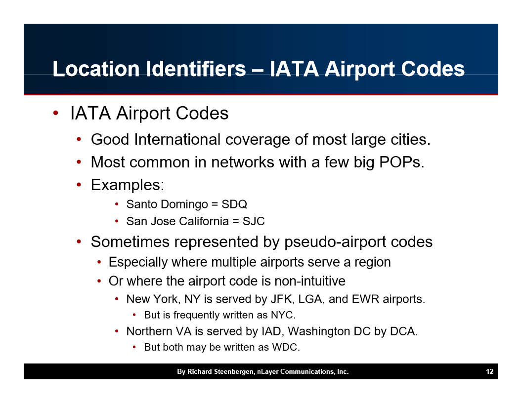
IATA codes (three-letter airport identifiers) are widely used in hostname conventions. For example, “AMS” refers to Amsterdam, “FRA” to Frankfurt, and “ORD” to Chicago.
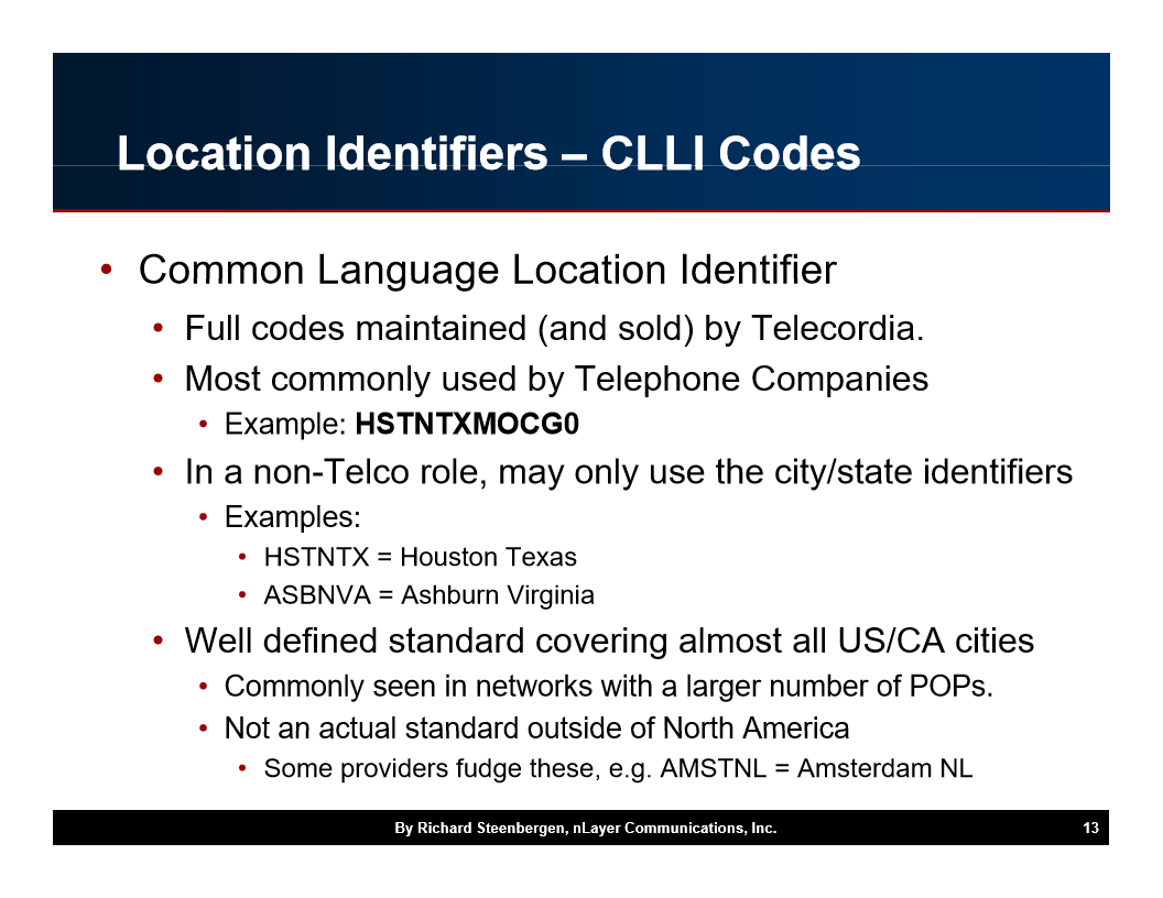
Common Language Location Identifiers
Some operators use plain city or region names in their hostnames, such as “ashburn,” “atlanta,” or “chicago.”
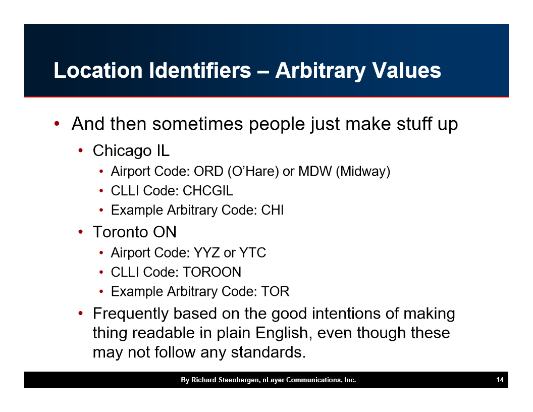
Arbitrary Values
Not every hostname is meaningful. Some operators use internal ticket numbers, build identifiers, or other arbitrary strings that will not help you identify the location.
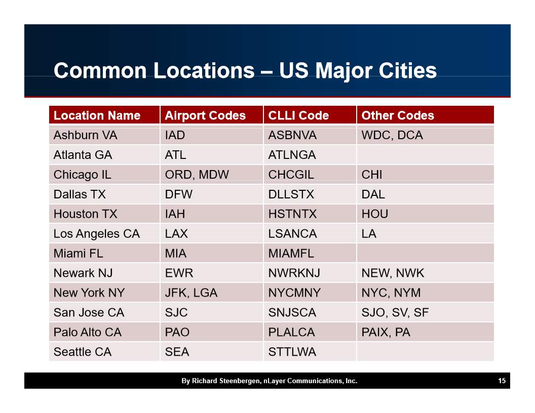
US Locations
Common US datacenter locations you will see in traceroute output include Ashburn VA, Atlanta GA, Chicago IL, Dallas TX, and others.
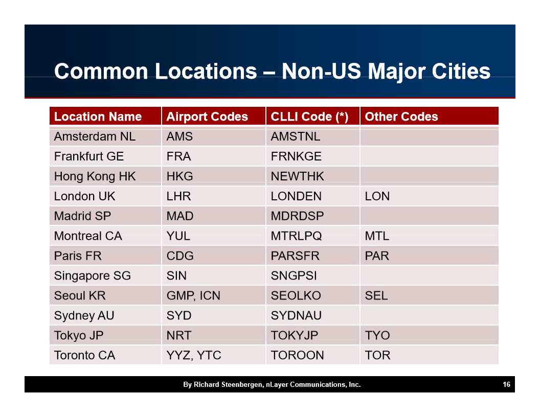
Non-US Locations
International locations follow similar patterns: Amsterdam NL, Frankfurt DE, London UK, and so on.
Interface Naming
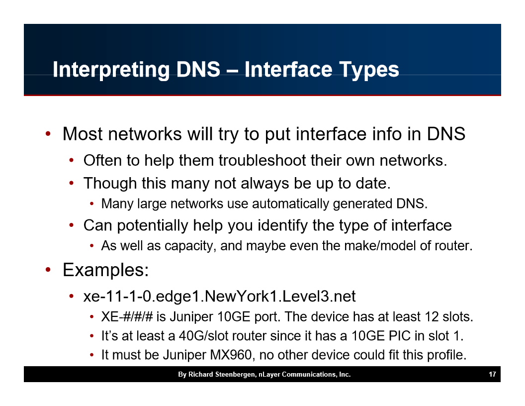
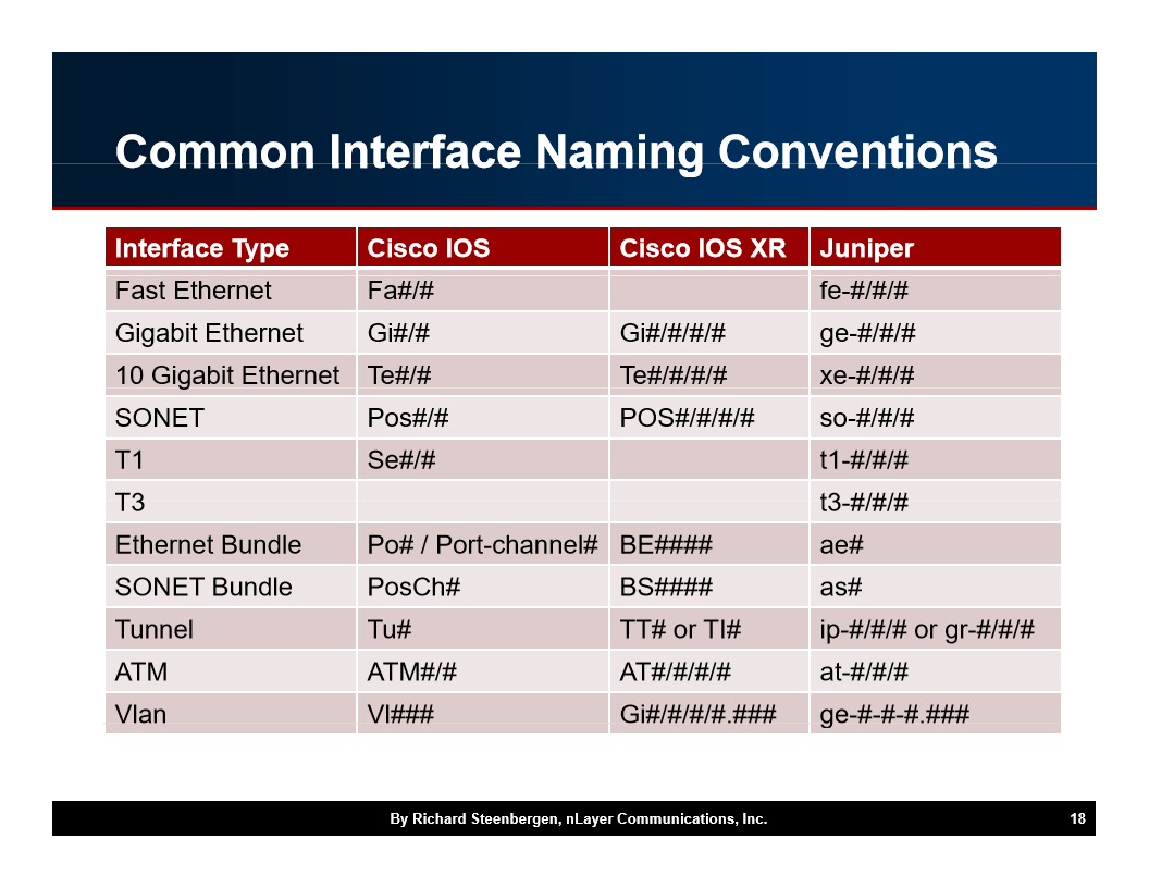
Hostnames often include the interface type and speed. For example, “Gi0/0/1” indicates a Gigabit Ethernet interface, while “Te0/1/0” indicates a 10 Gigabit Ethernet (or 100 Gigabit, depending on the vendor) interface.
Router Types and Roles
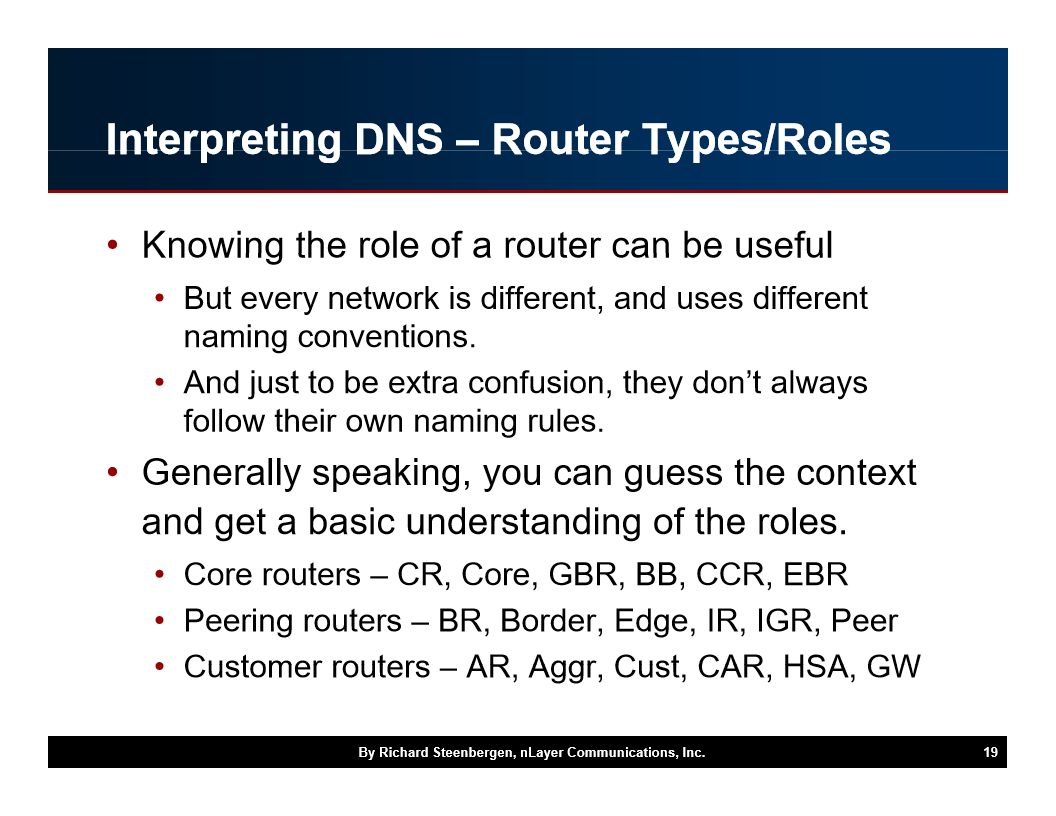
Knowing whether a hop is an edge router, a core router, or a peering router helps you understand where in the path you are. Edge routers typically face the customer or the internet; core routers handle high-volume transit.
Network Boundaries and Relationships
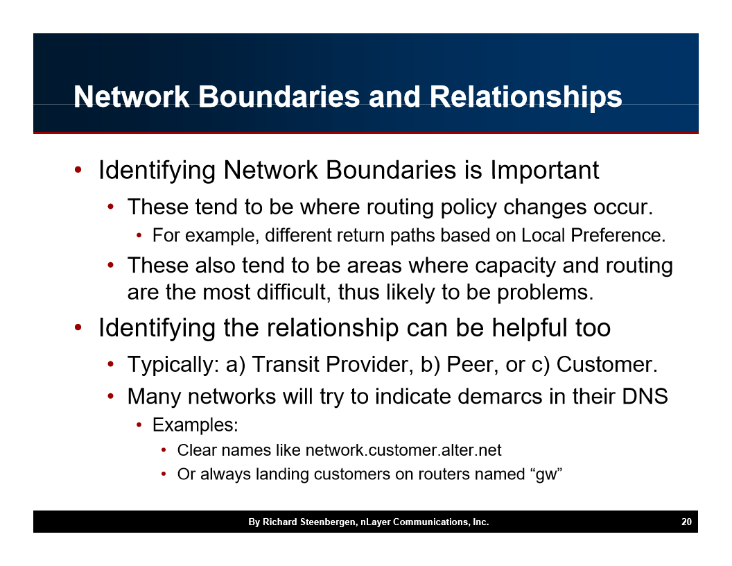
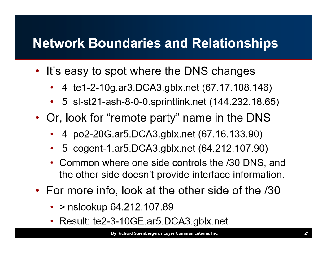
Identifying where one network ends and another begins is critical for understanding who owns a given hop and where a problem might originate.
Understanding Network Latency
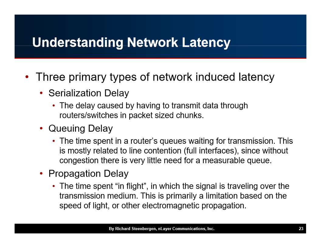
Latency in a network path is composed of three primary types of delay. Understanding each one helps you interpret traceroute numbers correctly.
Serialization Delay
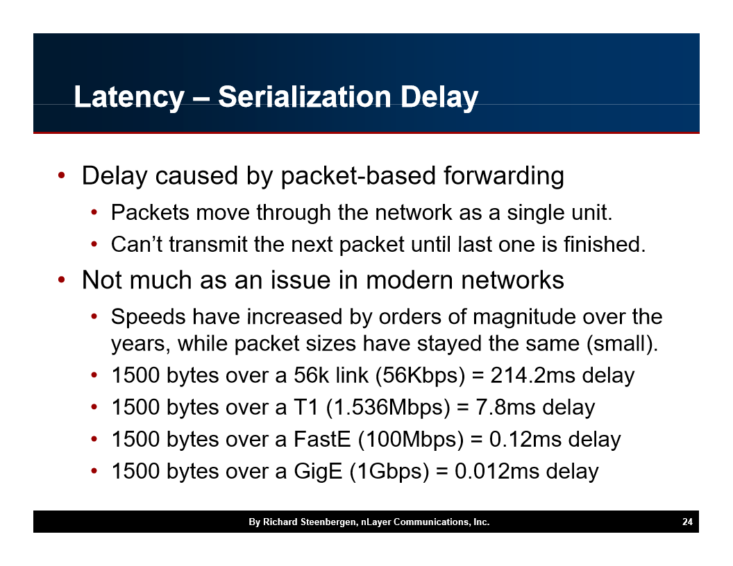
Serialization delay is the time it takes to push all the bits of a packet onto the wire. It is calculated as packet size divided by link speed. A 1500-byte packet on a 1 Gbps link takes roughly 12 microseconds to serialize.
Queuing Delay
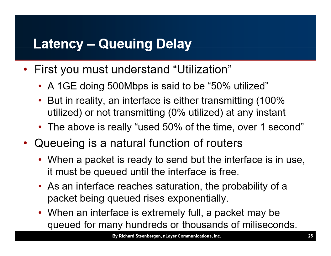
Queuing delay occurs when packets wait in a router’s buffer before being forwarded. Under normal load this is negligible, but during congestion it can add significant and variable delay.
Propagation Delay
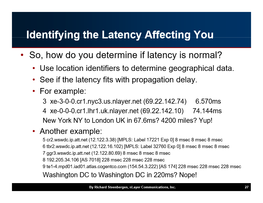
Propagation delay is the time it takes for a signal to travel the physical distance between two points. In fiber, light travels at roughly 200,000 km/s, so a 1000 km path adds about 5 ms of one-way propagation delay.

Identifying the Latency-Affecting Node
So how do you tell which hop is actually adding the delay you care about? Look for a consistent jump in RTT that persists across multiple probes and multiple traceroute runs. A single high reading is often just a slow ICMP response, not a real bottleneck.
Prioritization and Rate Limiting
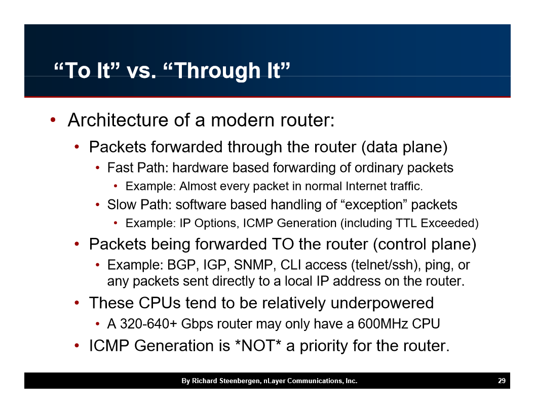
Modern routers do not treat all packets equally. Forwarded traffic gets top priority, while control-plane messages like ICMP Time Exceeded are deprioritized and often rate-limited.

The Infamous BGP Scanner
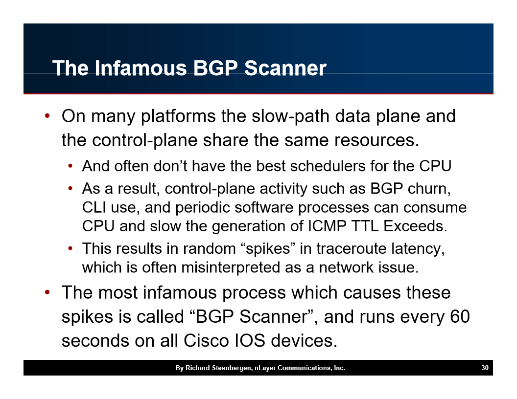
On many platforms, the slow path (CPU) handles BGP updates and other control-plane events. If the CPU is busy processing a BGP scan, ICMP responses can be delayed or dropped entirely, making a hop appear slow or unresponsive.
Rate-Limited ICMP Generation
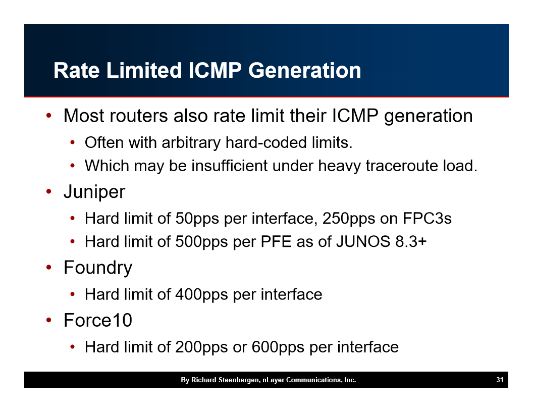
Most routers also rate-limit the generation of ICMP Time Exceeded messages. If you send probes faster than the rate limit allows, some will be silently dropped, and you will see asterisks or high latency in the output.
Spotting the Fake Latency
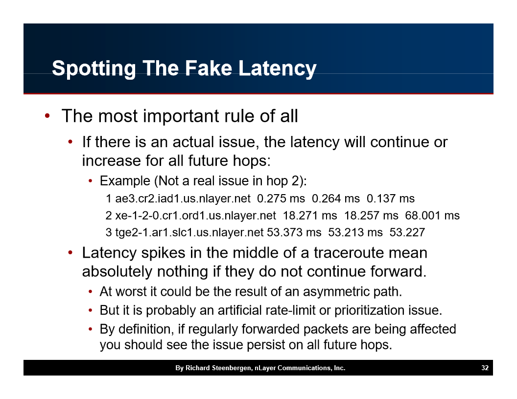
The most important rule: a high RTT at a single hop, especially if the next hop shows a lower RTT, is almost certainly a rate-limiting artifact, not a real network delay.
Asymmetric Paths
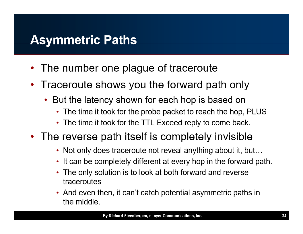
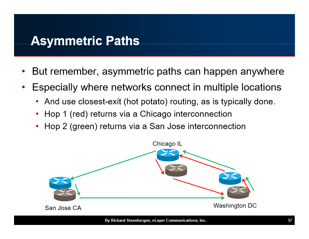
The number one plague of traceroute interpretation is asymmetric routing. The path your packets take to the destination may be different from the path the return ICMP messages take.

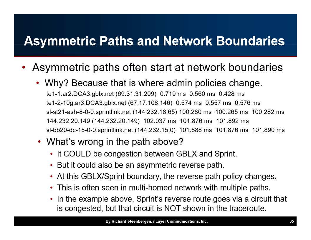
Asymmetric paths often start at network boundaries, where the forwarding table for outbound traffic differs from the table used for inbound traffic.
Using Source Address in Your Traceroute
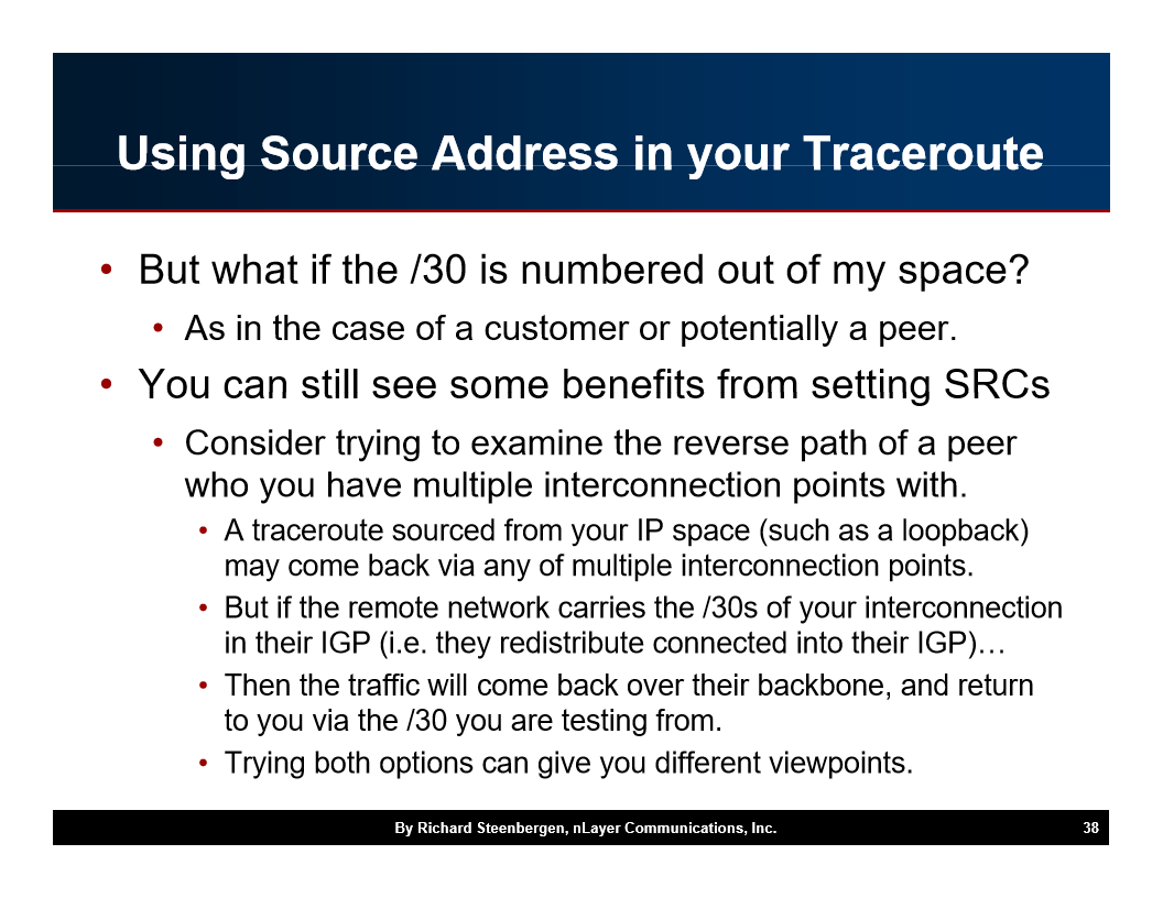
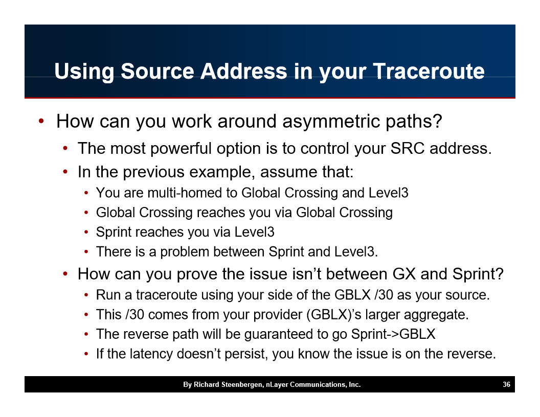
How can you work around asymmetric paths? One technique is to specify a source address that forces the traffic through a particular interface or path.
Default Source Address
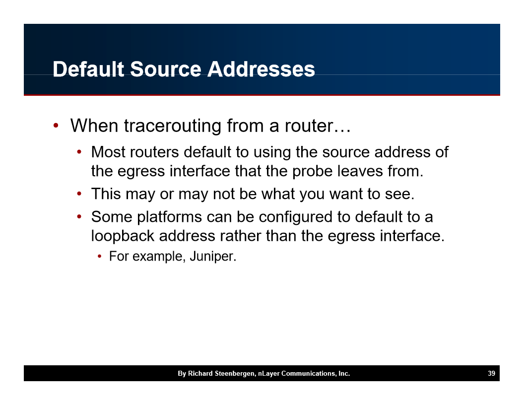
When tracerouting from a router, the default source address is the outgoing interface’s IP. If you have multiple interfaces facing the same destination, the source address you choose can change the path.
Multiple Paths and Load Balancing
Because each UDP or TCP traceroute probe may be load-balanced across multiple equal-cost paths, consecutive probes can take different routes. This is normal and does not indicate a problem.

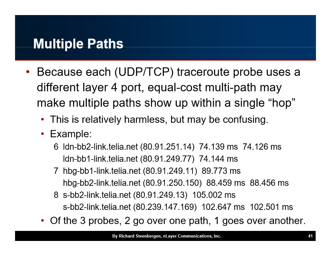
Multiple Paths Example
A slightly more complex example: if a router has two equal-cost paths to a destination, probe 1 might go via Path A while probe 2 goes via Path B. The output will show two different sets of hops interleaved.
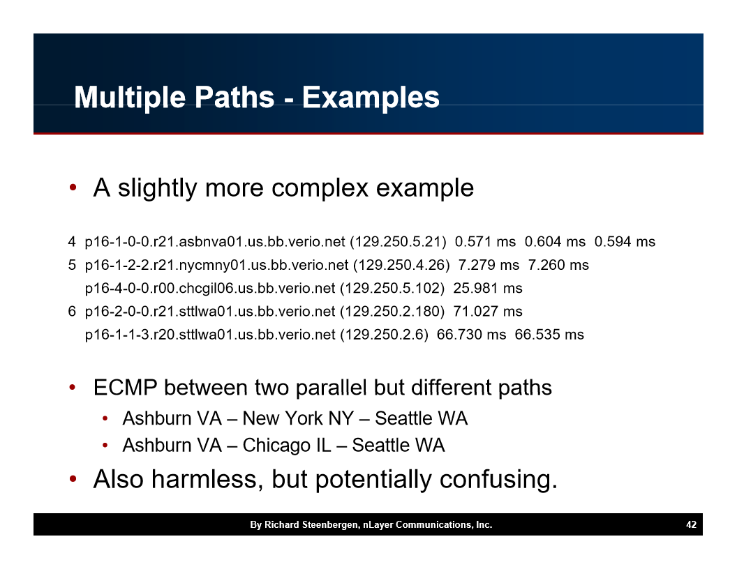
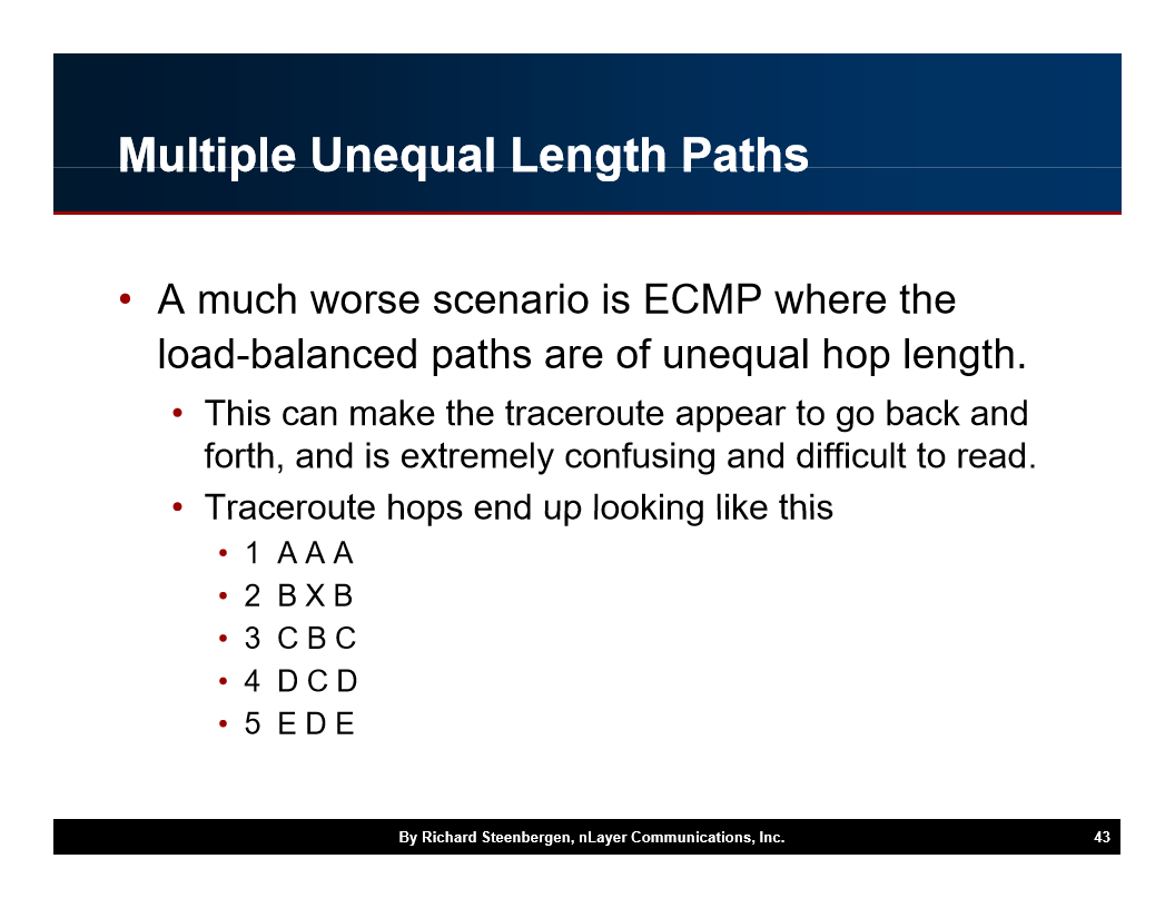
Multiple Unequal-Length Paths
A much worse scenario occurs when the two paths have different numbers of hops. The traceroute output can look confusing because the hop numbers do not align between the two paths.
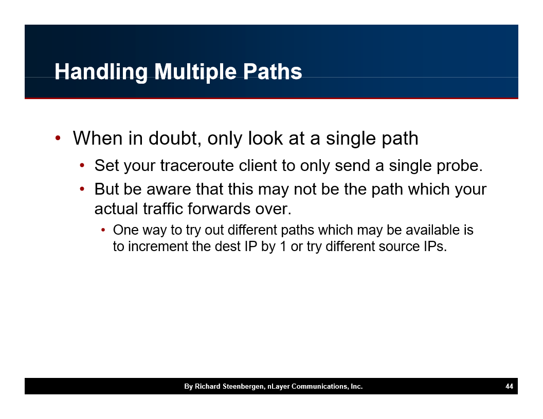
Handling Multiple Paths
When in doubt, only look at the hops that are consistent across all three probes. Inconsistent hops are likely load-balanced alternatives.
MPLS and Traceroute
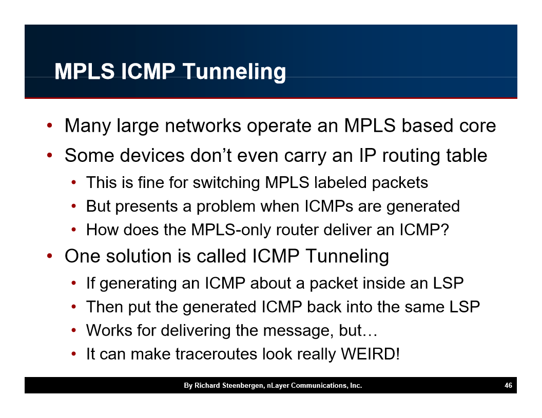
Many large networks operate an MPLS backbone. In these networks, traceroute output can show multiple hops for what is physically a single router, because each MPLS label operation (push, swap, pop) can generate a separate TTL-exceeded response.


Example Output
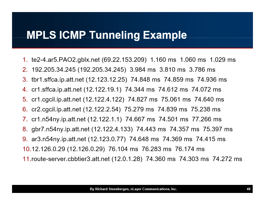
Here is a sample traceroute output showing the concepts discussed above:
Questions
Send questions, complaints, or corrections to Richard A. Steenberg, the original author of this guide.